Notes from Neural networks course

Lecture 0

Basics of Artifficial neural networks (NNs)

• primitive models – started in 50ties
  • like if a drunk neuroscientist and a programmer chatted in a bar about their fields
• NNs are data hungry
  • often other solution is way better (SVM, Dec. trees etc.)

Biological NN

• Humans have approx \(10^{11}\) neurons, \(10^4\) connections each
• Biological neurons are quiet until their electric potential is exceeded, then they “fire”
• Learning is believed to change the synaptic potential

Formal neuron

• \(x_1, ..., x_n \in \mathbb R\) are inputs

• TODO:

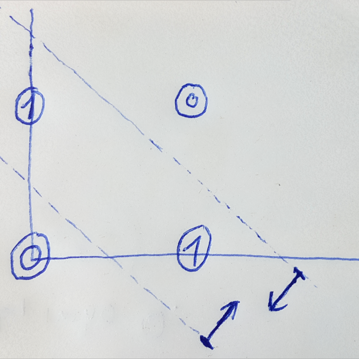
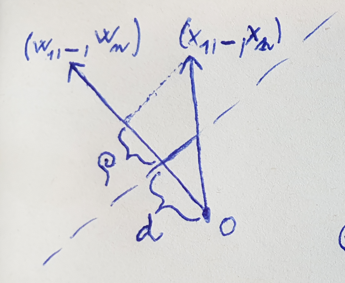
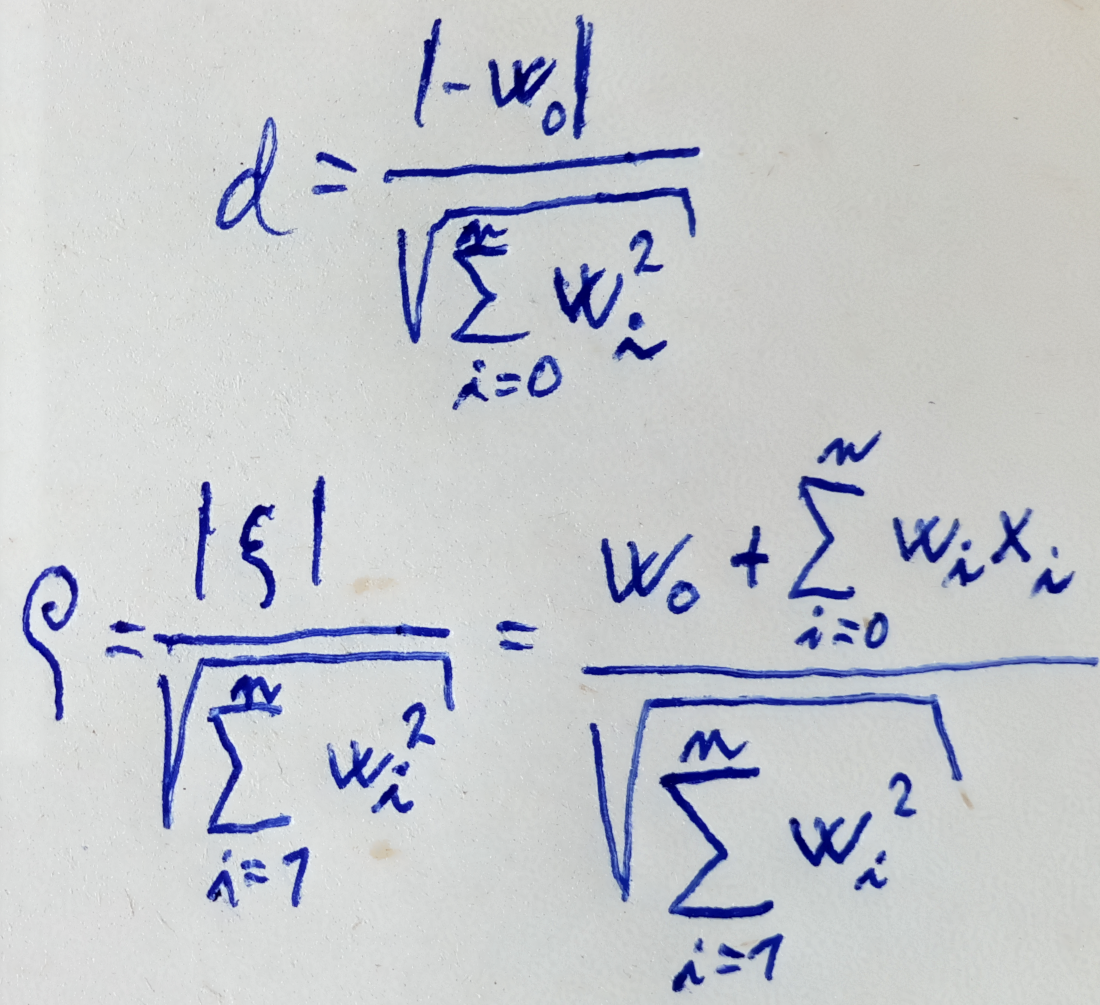
• Single neuron divides the hyperspace in “half” by a hyperplane
• The hyperplane is perpendicular to the weight vector

• Architecture – how the neurons are connected
• Activity – how the network transforms inputs to outputs

• Learning – how the weights transform

• Architecture example
  • Multilayer Perceptron (MLP)
    • Neurons in layers
    • Layers fully connected
• Activity
  • State – output values of a layer
  • State-space – set of all states
  • A computation is finite if there is finite number of steps

  • NN is a function: \(\mathbb R ^ n \rightarrow \mathbb R ^ m\)

  • Activation functions
    • Unit step function \(\sigma (\xi) = {1: \xi \geq 0; 0: \xi < 0}\)
    • (Logistic) sigmoid \(\sigma (\xi) = \frac 1 {1 + e ^ {-\lambda \cdot \xi}} \text{ here } \lambda \in \mathbb R \text{ is the steepness}\)
    • Hyperbolic tangens
  • XOR with 2 layer

• Learning
  • Configuration – vector of all values of weights
  • Weight-space – set of all (possible) configurations

  • Initial configuration

  • Supervised learning
  • Unsupervised learning
    • The goal is to determine distribution of the inputs by learning to reproduce -

FIX

Lecture 1

How strong are NN?

Boolean functions

• Any boolean function can be replicated by 2 layer NN

Any other function

1. Split the area into convex areas
2. Create tangents and “OR” them

or even stronger

1. Split into grid of (really small) squares
2. Any square is aproxitable with 4 neurons
3. “OR” all squares

Theorem – Cybenko (1989)

• They are strong: TODO

NN and computability

• Recurrent NN with rational weights are at least as strong as Turing machines
• Recurrent NN with irational weights are super-Turing machines (can decide Turing machines)

	Neural networks	Classical computers
Data	implicitly in weights	explicit
Computations	naturally parallel	sequential, localized*
Precision	imprecise	(typically) precise
Robustness	robust – 90+% can be deleted	fragile
TODO	✔	✔

How to learn NN (software)

• Tensorflow (Google) – highly optimized
  • Keras High level API
• Keras
• Theano – academic, clean, dead

Lecture 2

• \(E (w_0, ..., w_n) = \sum _ {i = 0}^n \frac {\delta} {w_i}\) TODO
• Why sigmoid as a loss function?
  1. let \(y\) be the probability of class A
  2. funciton of the odds: \(\frac {y} {1 - y}\)
  3. log it: \(\log \frac {y} {1 - y} = \vec w \cdot \vec x\)
  4. multiply by -1: \(\log \frac {1 - y} {y} = - \vec w \cdot \vec x\)
  5. move log: \(\frac {y} {1 - y} = e ^ {\vec w \cdot \vec x}\)
  6. stand alone \(y\): \(y = \frac 1 {1 + e ^ {\vec w \cdot \vec x}}\)

Lecture 3

MLP error fction gradient chain

• \[y_1 = o_1 (\xi _1 ); \xi _1 = w _{1, 2} \cdot y _2\]
• \[y_2 = o_2 (\xi _2 ); \xi _2 = w _{2, 3} \cdot y _3\]

• …

• Error for k: \(E_k = \frac 1 2 (y _ 1 - d _ {k _ 1}) ^ 2\)
• Derivatives:
  • \[\frac {\partial E_k} {\partial y _ 1} = y_1 - d_ {k _ 1}\]
  • \[\frac {\partial E_k} {\partial y _ 2} = \frac {\partial E_k} {\partial y _ 1} \cdot \frac {\partial y _ 1} { \partial \xi _ 1} \cdot \frac {\partial \xi _ 1} {\partial w _ {2, 3}} = \frac {\partial E_k} {\partial y _ 1} \cdot \sigma ' _1 (\xi _ 1) \cdot y _ 2\]
• Generalized:
  • \[\frac {\partial E _ k} {\partial w _ {j i}} = \frac {\partial E _ k} {\partial y _ j} \cdot \sigma ' _j (\xi _ j) \cdot y_i\]
  • trivial for j in last layer: \(\frac {\partial E_k} {\partial y _ 1} = y_1 - d_ {k _ 1}\)
  • otherwise: \(\frac {\partial E_k} {\partial y _ j} = \sum_{r \in \vec j} \frac {\partial E _ k} {\partial y _r} \cdot \sigma ' _r (\xi _ r) \cdot w _{rj}\)
• Derivations for different functions
  • logistic sigmoid: \(\sigma _j (\xi) = \frac 1 {1 + e ^ {-\lambda_j \xi}}\)
    • \[\sigma ' _j (\xi _ j) = \lambda _j y_j (1- y_j)\]
  • tanh:
• Computation: (exactly in slides)
  1. Forward pass
  2. Backward pass
  3. Compute derivation for all weights
     • the only place where we train the network using Gradient descent!
  • The steps 1–3 are linear with respect to the size of the NN
• Basically turn the network upside down and exchange weights with \(\sigma_x ' (\xi_x) \cdot w_{xy}\)

Lecture 4

Practical issues of SGD

• Training variables
  • Size of minibatch
  • Learning rate (and it’s decrease)
  • Pre-process of the inputs
  • Weights initialization
  • Output values
• Result quality check
  • When to stop
  • Regularization
  • Metrics

Not to forget when solving our own MNIST task

• TODO?

How to process BIG data

• Use minibatch – wouldn’t be random
  1. Split into subsets with equal distribution
  2. Train on each subset
  3. Shuffle all data
  4. Repeat 1.

Random claims

• With higher dimension, different inicialization will get
• It’s easy to get stuck in a flat place, especially if using the Sigmoid function
• It’s typical to choose power of 2:
  • The bigger, the better – theoretically
  • The smaller the better (32 to 256) – empirically

Issues

Vanishing and exploding gradients

• \[\frac {\partial E_k} {\partial y _j} = \sum _ {r \in j^ \rightarrow} \frac {\partial E_k} {\partial y _r} \cdot \sigma '_r (\xi _r) \cdot w_{rj}\]
  • Every layer in the back propagation multiplies by a number under 1
  • The “signal” going back is getting lower and lower =>
  • We may truly train just the last few layers in a very big network

Moment

• Gradient descent ( \(\nabla E(w)\) TODO…) changes the direction with every step a lot
• Solution: In every step of G. descent add a part of the direction you were going from

Learning rate

• “The single most influential hyperparameter.”

TODO: Img from the presentation

1. Use scheduler
2. Lower the rate
3. Use different optimizer

AdaGrad

• parameter-specific learning rates, which are adapted relative to how frequently a parameter gets updated during training.

• The more updates a parameter receives, the smaller the updates.

• Problem: r get bigger and bigger

RMSprop

• Like AdaGrad, but forgets the past

Adam

• Like RMSprop, but with build-in momentum

Choice of (hidden) activations

1. differenctiability
   • for gradient descent
2. non-linearility
   • linear * linar = linear
3. monotonicity
   • do not add more local extrems
4. “linearity”
   • linear-like functions are easier (derivations, learning speed..)

Before training

Range not around 0

• Typical standardization:
  1. Average = 0 (subtract the mean)
  2. Variance = 1 (divide by the standard deviation)

Initial weights

• We want to have the standard
• Too small \(w\) we get (almost) linear model

• Too large \(w\) we get to the saturated regions (binary?)

• \[o_j = \sqrt \frac d 3 \cdot w\]
• Therefore: \(w = (- \frac {\sqrt 3} {\sqrt d}, \frac {\sqrt 3} {\sqrt d})\)
  • Where \(d\) is # of input weights

• The forward pass is nice, but back propagation can Explode

• How does this interfere with Dropout?

Glorot & Belgio initialization (GLOROT)

• \[(- \sqrt \frac 6 {m + n}, \sqrt \frac 6 {m + n})\]
• Takes in count both sides of the neuron (m = # of inputs, n = # of outputs)
• Should work better even for back propagation

Output neurons

• Regression: linear or sigmoid
• Binary classification: tanh or sigmoid
• N classification: softmax
• Multiple classes: sigmoidal outputs and classes individually

Lecture 5

Generalization

• Data has, in general, some noise in it
• We don’t want to learn the noise

Overfitting

“With four parameters I can fit an elephant, with five I can make him wiggle his trunk.” – John Von Neumann

• What can we overfitt with GB of parameters?

Early stopping

• Split into
  • Training set (train the network)
  • Validation set (use to stop the training)
  • Test set (evaluation)
  • Never ever seen data (do not even look at them)

Sigmoidal & cross-entropy

• It’s (generaly) bad idea to use Sigmoidal + MSError
  • The derivation is symetrical, so if you are completely wrong (or right), the error is small
• Cross-entropy solves this
  • The error is big when the prediction is completely wrong and small only when you are almost right

Ensemble methods

• The idea: train several different models separately, then have all of the models vote on the output for test

Dropout

• Include the Ensemble method into one network
• Original implementation:
  • In every step of SGD, every neuron is included with \($ \frac 1 2\)$ probability
• Modern: just randomly choose X % of the neurons of the layer
• Usually used without L2 norm

Weight decay and L2 regularization

• Push on the weights, make them prove themselves

• In every step, decrease weights

• L1 norm – (probably) good for sparsity
• L2 norm – penalizes large weights, theoretically the same
  • Usually used without Dropout

Convolutional layers

• Extracts features, read elsewhere

Pooling

• Max-pooling: max of inputs
• L2 … # TODO

Dataset expansion

• Move by \($x\)$ pixels to all directions
• Add noise
• Distort images (especially for Health data)
• => able to create 100 000 examples from only 1000

-

.

.

.